Medium-Range Weather Forecasting with Time- and Space-aware Deep Learning Part 1: History
Machine learning models now outperform the best numerical weather prediction systems. But the theory underlying their impressive performance is as old as numerical weather prediction itself.
This is the first post in a multi-post series on emerging deep learning methods for medium-range weather forecasting. The full and most recent version of this review can be found here.
The Birth of Numerical Weather Prediction
In 1922, the English mathematician Lewis Fry Richardson published a book detailing the boundaries of the field of numerical weather prediction (NWP) nearly a half a century before it would actually take shape, cementing himself as one of the most prescient scientific minds in history. Richardson’s first and only book-length work, Weather Prediction by Numerical Process (WPNP) (Richardson, 1922), is an ingenious, Turing-like blend of mathematical science and technological fiction which spelled out—with near-perfect foresight—how global weather patterns would someday be predictable if the computational and observational infrastructure were built to support it. While this infrastructure has evolved over the proceeding century from fantasy to public utility and now public utility to downloadable AI model, Richardson’s insights about the spatial and temporal constraints which govern NWP have remained at the theoretical core of each iteration.
Inspired by earlier meteorologists like Abbe and Bjerknes who posited that weather events may be explainable based on hydrological and thermodynamic properties of the atmosphere, the majority of WPNP is traversed by a labyrinthine collection of partial differential equations which are hypothesized to govern the behavior of a wide variety of atmospheric variables like pressure, temperature, water content, or wind direction. While most of these governing equations were well-known to the meteorological community at the time, the genius of WPNP derives from the book’s integration of these atomic physical equations into a system for weather forecasting which, by simulating the future value of a collection of equations based on initial observations of the weather’s state, could forecast the weather within a geographic area from physical first principles.
Richardson assumed that the state of the weather could be approximated by seven partial differential equations governing atmospheric pressure, temperature, density, water content, and the three directional velocity components wind. He imagined these variables to be measurable along a “chequering” of points patterned across the Earth’s surface which divided the atmosphere into columns of 3° east-west and 200 km north-south, 12,000 columns circling the globe. Each of these columns were divided horizontally by four lines, creating a grid pattern. From this chequering, the solution to each governing equation could be approximated in finite difference form and then propagated forward in time, producing a forecast of future weather based on the current conditions reported within each chequer.
Richardson’s spatial grid used to solve for atmospheric variables in his example forecast. This approach to discretizing the globe and solving for future weather patterns based on the spatial interactions of weather across grid points underlies modern weather forecasting. (Richardson 1922).
The initial distribution of weather observations on Richardson’s example grid. Each chequer contains weather observations at a point in time. These observations are then projected forward to produce a weather forecast by solving a system of differential equations. A grid of observations like this is the primary input data structure to modern weather forecasting. (Richardson 1922).
The majority of WPNP functions as a rote review of the differential equations governing the temporal relationships of the atmospheric variables in Richardson’s model. This technical review appears at first to meander, jumping between ideas in mathematically-condensed language. It isn’t until the ninth chapter, 180 pages into the book, that we are able to reinterpret the earlier chapters not as aimless mathematical statements, but the requisite elements for a tightly-wound computational forecasting system. With the background theory finally in place, nearly three-quarters of the way through the book the tone shifts to that of a field journal, documenting the manual calculations of the first modern numerical weather prediction system. In this calculation, Richardson produces a 6-hour forecast of initial changes of the atmospheric mass and wind variables from a collection of initial state estimations over a small chequering of Europe centered near Munich. He writes,
The process described in Ch. 8 has been followed so as to obtain [the partial derivative with respect to time] of each one of the initially tabulated quantities.
The arithmetical accuracy is as follows. All computations were worked twice and compared and corrected. The last digit is often unreliable, but is retained to prevent the accumulation of arithmetical errors. Multiplications were mostly worked by a 25 centim slide rule.
The rate of rise of surface pressure, [the partial derivative of pressure with respect to time] is found on Form PXIII as 145 millibars in 6 hours, whereas observations show that the barometer was nearly steady. This glaring error is examined in detail below in Ch. 9/3…
Despite expending significant manual effort in compiling the observational estimates, computing the forecast, and double-checking the calculations, Richardson’s forecast predicted an unrealistic 145hPa change in pressure over Munich within 6 hours, resulting in an approximate 145 root mean-squared error (RMSE) value for his forecasting accuracy. While his other variable calculations were less extreme, this forecasting failure was cited by many meteorologists at the time as reason to dismiss Richardson’s proposed numerical approach to weather prediction (Lynch, 2022).
The dismissal of his work by contemporaries based on the miserable results of this first numerical approach to weather forecasting proved to be immensely short-sighted. In WPNP’s penultimate chapter Richardson, now unburdened by empirical failure to continue discussing his tractable model, offers his projection of how this model for weather forecasting may be scaled in the future, and ends up producing one of the most clairvoyant works of science fiction in the process. In this chapter titled “Some Remaining Problems”, Richardson hones in on the spatio-temporal computational constraints which continue to dictate the structure of numerical weather computing to this day:
It took me the best part of six weeks to draw up the computing forms and to work out the new distribution in two vertical columns for the first time. My office was a heap of hay in a cold rest billet. With practice the work of an average computer might go perhaps ten times faster. If the time-step were 3 hours, then 32 individuals could just compute two points so as to keep pace with the weather, if we allow nothing for the very great gain in speed which is invariably noticed when a complicated operation is divided up into simpler parts, upon which individuals specialize. If the co-ordinate chequer were 200 km square in plan, there would be 3200 columns on the complete map of the globe. In the tropics the weather is often foreknown, so that we may say 2000 active columns. So that 32 x 2000 = 64,000 computers would be needed to race the weather for the whole globe. That is a staggering figure. Perhaps in some years’ time it may be possible to report a simplification of the process. But in any case, the organization indicated is a central forecast-factory for the whole globe, or for portions extending to boundaries where the weather is steady, with individual computers specializing on the separate equations. Let us hope for their sakes that they are moved on from time to time to new operations.
From his tedious experience producing a numerical weather prediction by hand, Richardson understood intimately that numerical weather prediction amounts to a race against time: forecasting the weather in 6 hours is useless if the forecast takes longer than that to produce. He was also keen to point out that global weather forecasting would become a computationally expensive process whose scale would be determined by the fidelity of the computational grid that anchor the observations and forecasts across the Earth’s surface. Richardson’s imaginative prophecy continues:
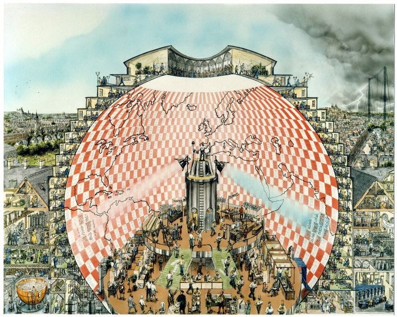
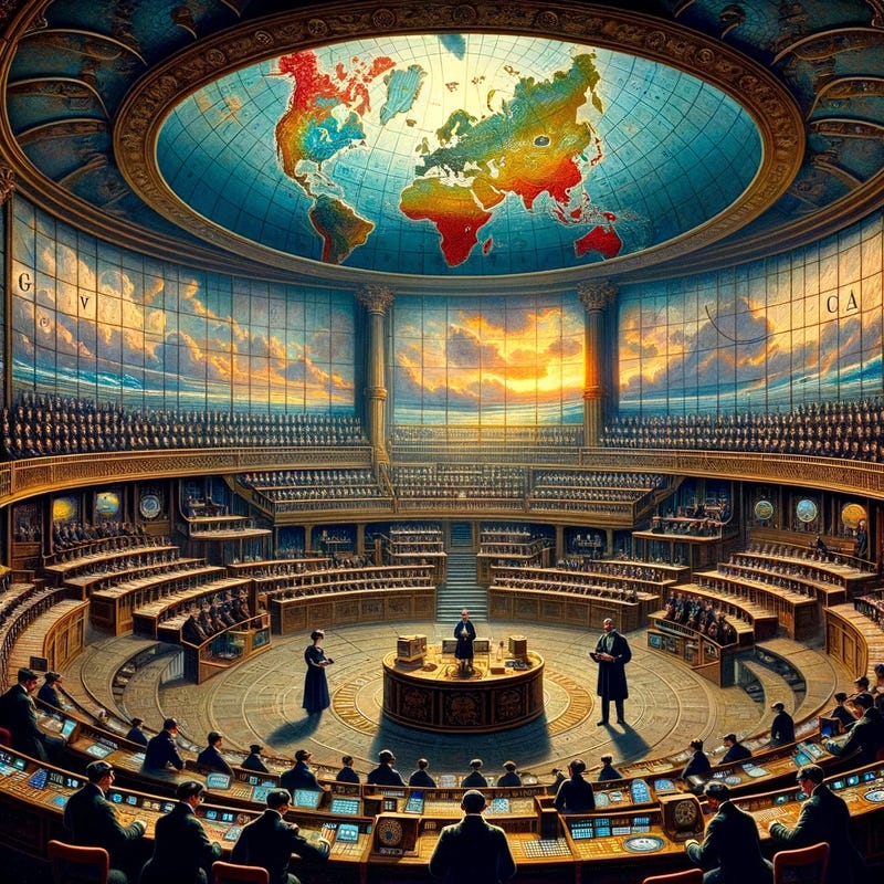
After so much hard reasoning, may one play with a fantasy? Imagine a large hall like a theatre, except that the circles and galleries go right round through the space usually occupied by the stage. The walls of this chamber are painted to form a map of the globe. The ceiling represents the north polar regions, England is in the gallery, the tropics in the upper circle, Australia on the dress circle and the antarctic in the pit. A myriad computers are at work upon the weather of the part of the map where each sits, but each computer attends only to one equation or part of an equation. The work of each region is coordinated by an official of higher rank. Numerous little night signs display the instantaneous values so that neighbouring computers can read them. Each number is thus displayed in three adjacent zones so as to maintain communication to the North and South on the map. From the floor of the pit a tall pillar rises to half the height of the hall. It carries a large pulpit on its top. In this sits the man in charge of the whole theatre ; he is surrounded by several assistants and messengers. One of his duties is to maintain a uniform speed of progress in all parts of the globe. In this respect he is like the conductor of an orchestra in which the instruments are slide-rules and calculating machines. But instead of waving a baton he turns a beam of rosy light upon any region that is running ahead of the rest, and a beam of blue light upon those who are behindhand.
Note the spatial and message-passing structure implicit in Richardson’s weather theatre fantasy. Each computer (a person, in his time) was tasked with the computations related to a particular chequer, but these computations would both influence and would be influenced by the computational results derived from its neighboring computers. Richardson imagines these spatially distributed calculations to be carried out in time, with short-range forecasts feeding into those at longer ranges.
Richardson’s forecast theatre, as illustrated by Stephen Conlin (1986).
Richardson’s forecast theatre, as illustrated by Dall-E 3 (Betker et al. 2023).
As will become clear in the following sections, the spatio-temporal computing patterns imagined by Richardson to drive the weather forecasting in his fantasy theatre are exactly those which have come to dominate the structure of NWP over a century into the future. Moreover, these same spatio-temporal constraints are being used as the foundation to a new approach to NWP using spatially-biased deep learning architectures from the field of machine learning. Indeed, Richardson’s fantasy is as relevant today as it has ever been.
While Richardson himself never saw the construction of his forecast theatre, in time it was eventually built, and its complexity grew with each passing decade. What Richardson couldn’t have predicted, however, is that the physical size of his theatre would eventually become uncoupled from this complexity. With the introduction of AI models in NWP, Richardson’s theatre now fits on a single GPU.
An Early Benchmark
Richardson died in 1953, still decades before the emergence of a global, real-time numerical weather prediction system at the scale imagined in his fantasy. However, he did live long enough to observe the first major steps towards this system: the results of the first numerical weather predictions implemented on an digital computer. In 1950, Charney, Fjortoft and von Neumann calculated a forecast of atmospheric flow on the ENIAC, the first programmable, general-purpose computer (Charney, Fjörtoft, & Neumann, 1950). While their forecast was concerned with integrating the barotropic vorticity equation alone, their approach drew clear inspiration from Richardson’s work, including the use of a grid of points to anchor the differential equation. Shortly after publication, Charney shared his results, published in Tellus, with Richardson. In response, Richardson congratulated Charney on the “remarkable progress which has been made at Princeton” (Platzman, 1968). Included in his response, however, was an intriguing new analysis:
I have today made a tiny psychological experiment on the diagrams in your Tellus paper of November 1950. The diagram c was hidden by a card, which also hid the legend at the foot of the diagrams. The distinctions between a, b and c were concealed from the observer, who was asked to say which of a [initial map] and d [computed map 24 hours later] more nearly resembled b [observed map 24 hours later]. My wife’s opinions were as follows:
Thus d has it on the average, but only slightly. This, although not a great success of a popular sort is anyways an enormous scientific advance on the single, and quite wrong, result in which Richardson (1922) ended.
Richardson provided his wife, Dorothy Garnett, with a map of the initial observations of the variable being predicted (a), the 24 hours forecasted variable from the model mapped to the same grid (d), and the actual observation read 24 hours in the future. From this, Dorothy determined that the model forecast slightly outperformed a simple 1-day autoregressive baseline model, a benchmark called persistence in modern parlance. This analysis likely makes Dorothy Garnett the first person to ever benchmark a NWP weather model. And she did a good job. A 2008 re-creation of the Tellus forecast showed that Dorothy’s eyeballed evaluations were approximately in-line with modern quantitative metrics of forecast skill (Lynch, 2008), metrics we will make significant use of in the course of this review.
Charney was greatly encouraged by the Richardsons’ response to the Tellus work, and devoted time over the following year to honing his group’s algorithmic approximation of barotropic vorticity. Convinced his new results would sweep the Richardsons’ scorecard, he sent an updated version of the paper figures to Richardson in late 1953. Richardson died five days before the reprint arrived (Platzman, 1968).
References
Richardson, L. F. (1922). Weather prediction by numerical process. University Press.
Lynch, P. (2022). Richardson’s forecast: The dream and the fantasy. arXiv Preprint arXiv:2210.01674.